Constructing the Jones polynomial to save the world
Day 0: smalltowns-ville, IA:
A man picks up his daily slice of breakfast pizza from his local gas station. What he doesn’t know is that it’s his last. By mid-day he feels terrible, by the time he’s ready to go home for dinner he’s already feasting on brains.
Day 4: CDC Headquarters
The Z-virus has spread midwest-wide. You’re working at the CDC as an expert in microscopy. You’re working frantically to get any information on the Z-virus you can. You decide to image the DNA of the Z-Virus.
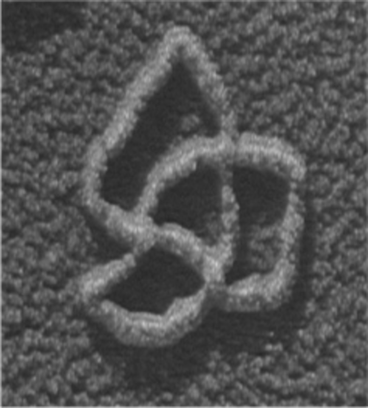
DNA knot as seen under the electron microscope. - Image Credit: Javier Arsuaga,
CC BY-ND
DNA
Deoxyribonucleic acid (abbreviated DNA) is the molecule that carries genetic information for the development and functioning of an organism.
DNA is made of two linked strands that wind around each other to resemble a twisted ladder — a shape known as a double helix.
Each strand has a backbone. Attached to each sugar is one of four bases: adenine (A), cytosine (C), guanine (G) or thymine (T). The two strands are connected by chemical bonds between the bases: adenine bonds with thymine, and cytosine bonds with guanine.
Vinograd, J., Lebowitz, J., Radloff, R., Watson, R., & Laipis, P. (1965) discover that double-stranded DNA can “supercoil”.
Vinograd, J., Lebowitz, J., Radloff, R., Watson, R., & Laipis, P. (1965). The twisted circular form of polyoma viral DNA. In Proceedings of the National Academy of Sciences (Vol. 53, Issue 5, pp. 1104-1111). Proceedings of the National Academy of Sciences.
https://doi.org/10.1073/pnas.53.5.1104
Day 7: CDC Headquarters
The spread is now nation wide but still under some control.
You’ve successfully imaged the DNA of the Z-virus and found DNA with a knot. Your CDC coworkers are using your findings to construct an anti-Z-virus. The anti-virus is the mirror of the DNA knot you’ve found. This will allow the human body to build anti-bodies for the Z-virus.
The CDC now needs you to verify that the DNA knot they’ve produced truly is the mirror of the Z-virus.
Anti-Knot
$\ $
Mathematical Knots
“A knot is a smooth embedding of a circle $S^1$ into Euclidean 3-dimensional space $\R^3$ (or the 3-dimensional sphere $S^3$ ).”
$\quad$
$\quad$
$\quad$
Jablan, S., & Sazdanović, R. (2007). Linknot. In Series on Knots and Everything. WORLD SCIENTIFIC.
https://doi.org/10.1142/6623
We want to use our bracket to build a polynomial that can tell two knots apart.
In particular, we want to differentiate a knot and its “anti-knot”(mirror).
Putting pieces together
How can we tell two knots apart?
How can we use that and our bracket to build our polynomial?
Check what happens under Reidemeister moves
If our bracket “respects” Reidemeister moves it respects knot “equivalence”.
Time is running out. With your preliminary results in hand the vaccine is being produced. The future of the world is now on your shoulders waiting for your results.
With the successful completion of your work the vaccine is being administer world wide. The President congratulates you for your work and the world is optimistic.
Day 300
The virus is completely controlled and you win every prize in every field imaginable!
The Jones Polynomial
The Jones Polynomial $V\LP \mathscr{K}\RP$ of an oriented knot $\mathscr{K}$
is the Laurent polynomial with integer coefficients in $t^{1/2}$.
Defined by
$ V\LP \mathscr{K}\RP=\LP\LP-A\RP^{-3w(P)}\LA P\RA\RP _{t^{1/2}=A^{-2}} $
where $P$ is any oriented diagram for $\mathscr{K}$.
Dale Rolfsen, Knots and links, Mathematics Lecture Series, vol. 7, Publish or Perish, Inc., Houston, TX, 1990, Corrected reprint of the 1976 original.
Robert Glenn Scharein. Interactive topological drawing. ProQuest LLC, Ann Arbor, MI, 1998. Thesis Ph.D. The University of British Columbia (Canada). URL:
https://www.knotplot.com/.
Jablan, S., & Sazdanović, R. (2007). Linknot. In Series on Knots and Everything. WORLD SCIENTIFIC.
https://doi.org/10.1142/6623
DNA knot as seen under the electron microscope. - Image Credit: Javier Arsuaga,
CC BY-ND
Vinograd, J., Lebowitz, J., Radloff, R., Watson, R., & Laipis, P. (1965). The twisted circular form of polyoma viral DNA. In Proceedings of the National Academy of Sciences (Vol. 53, Issue 5, pp. 1104-1111). Proceedings of the National Academy of Sciences.
https://doi.org/10.1073/pnas.53.5.1104